How to perform validation?

The following code performs computation of \(\alpha\) and \(\beta\) diversity from field plots and extracts the corresponding diversity indices from previouly computed SpectralSpecies raster in order to perform validation.

# location of the directory where shapefiles used for validation are saved
VectorDir <- destunz
# list vector data
Path_Vector <- list_shp(VectorDir)
Name_Vector <- tools::file_path_sans_ext(basename(Path_Vector))
# location of the spectral species raster needed for validation
Path_SpectralSpecies <- Kmeans_info$SpectralSpecies
# get diversity indicators corresponding to shapefiles (no partitioning of spectral dibversity based on field plots so far...)
Biodiv_Indicators <- diversity_from_plots(Raster_SpectralSpecies = Path_SpectralSpecies, 
                                          Plots = Path_Vector,
                                          nbclusters = nbclusters, 
                                          Raster_Functional = PCA_Output$PCA_Files, 
                                          Selected_Features = Selected_Features)

Shannon_RS <- c(Biodiv_Indicators$Shannon)[[1]]
FRic <- c(Biodiv_Indicators$FunctionalDiversity$FRic)
FEve <- c(Biodiv_Indicators$FunctionalDiversity$FEve)
FDiv <- c(Biodiv_Indicators$FunctionalDiversity$FDiv)
# if no name for plots
Biodiv_Indicators$Name_Plot = seq(1,length(Biodiv_Indicators$Shannon[[1]]),by = 1)

The diversity indices corresponding to the plots can then be written in CSV files.

# write a table for Shannon index
Path_Results <- file.path(Output_Dir,NameRaster,TypePCA,'VALIDATION')
dir.create(Path_Results, showWarnings = FALSE,recursive = TRUE)
write.table(Shannon_RS, file = file.path(Path_Results,"ShannonIndex.csv"),
            sep="\t", dec=".", na=" ", row.names = Biodiv_Indicators$Name_Plot, col.names= F,quote=FALSE)

# write a table for all spectral diversity indices corresponding to alpha diversity
Results <- data.frame(Name_Vector, Biodiv_Indicators$Richness, Biodiv_Indicators$Fisher,
                      Biodiv_Indicators$Shannon, Biodiv_Indicators$Simpson,
                      Biodiv_Indicators$FunctionalDiversity$FRic,
                      Biodiv_Indicators$FunctionalDiversity$FEve,
                      Biodiv_Indicators$FunctionalDiversity$FDiv)

names(Results)  = c("ID_Plot", "Species_Richness", "Fisher", "Shannon", "Simpson", "FRic", "FEve", "FDiv")
write.table(Results, file = file.path(Path_Results,"AlphaDiversity.csv"),
            sep="\t", dec=".", na=" ", row.names = F, col.names= T,quote=FALSE)

# write a table for Bray Curtis dissimilarity
BC_mean <- Biodiv_Indicators$BCdiss
colnames(BC_mean) <- rownames(BC_mean) <- Biodiv_Indicators$Name_Plot
write.table(BC_mean, file = file.path(Path_Results,"BrayCurtis.csv"),
            sep="\t", dec=".", na=" ", row.names = F, col.names= T,quote=FALSE)

These results can then be displayed according to the need for further analysis.

Here, for the purpose of illustration, we provide a code in order to visualize the differences among field plots located in the image: we first perform a PCoA on the Bray Curtis dissimilarity matrix computed from the field plots:

# apply ordination using PCoA (same as done for map_beta_div)
library(labdsv)
MatBCdist <- as.dist(BC_mean, diag = FALSE, upper = FALSE)
BetaPCO <- pco(MatBCdist, k = 3)

The plots corresponding to forested areas with high, medium and low diversity, as well as low vegetation/degraded forest close tomain roads are distributed as follows:

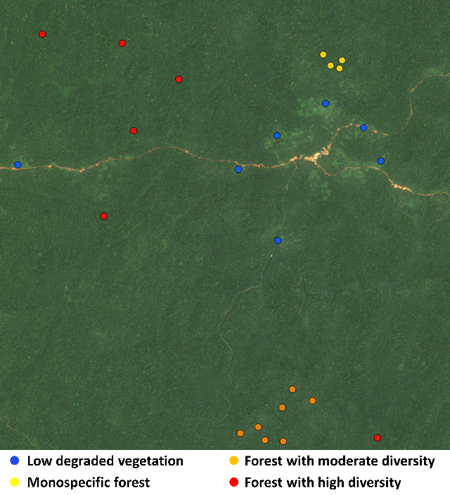
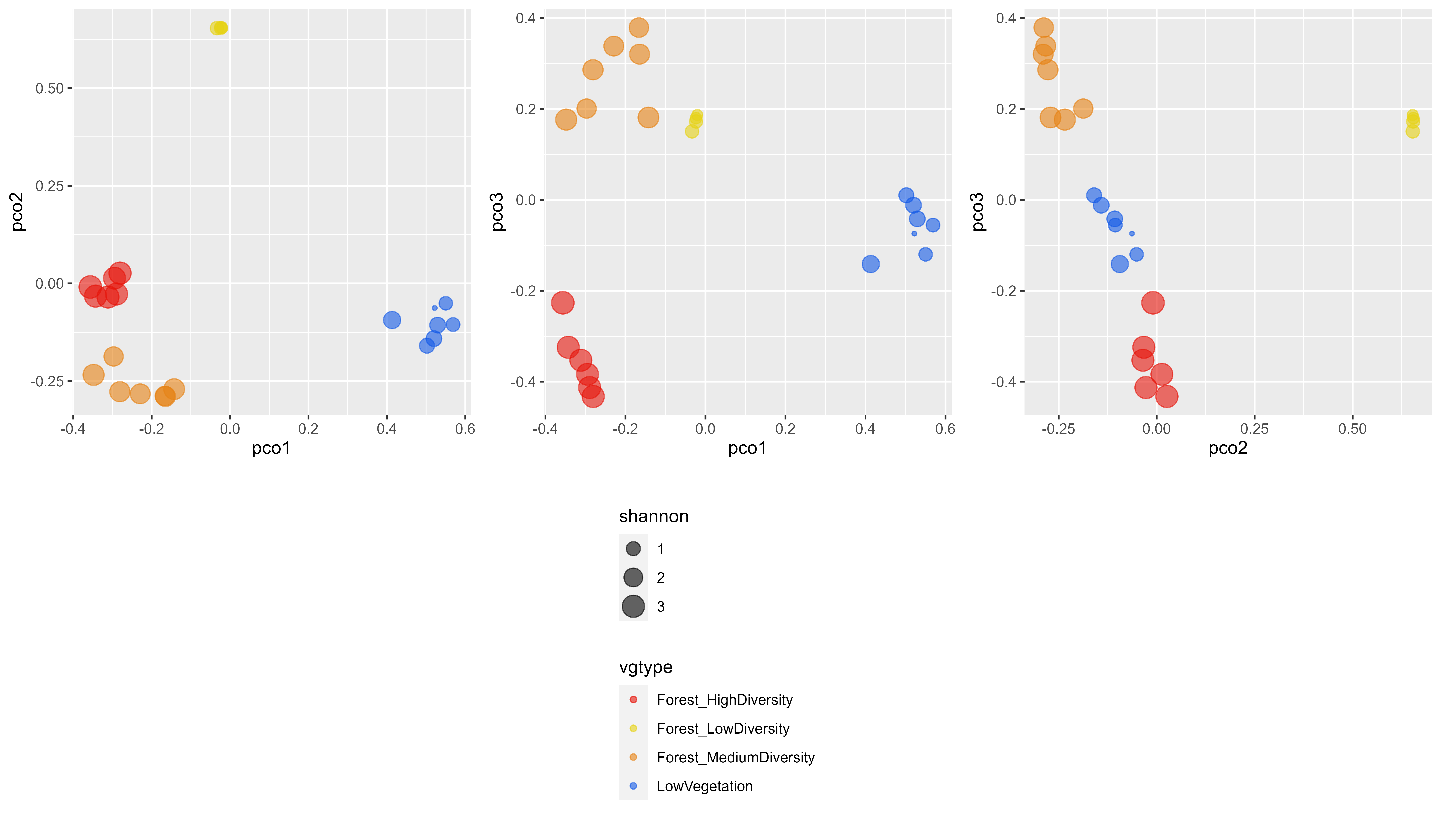
Here, we produce figures in order to locate the different types of vegetation in the PCoA space:

# assign a type of vegetation to each plot, assuming that the type of vegetation 
# is defined by the name of the shapefile
library(terra)
library(tools)
library(ggplot2)
library(gridExtra)
nbSamples <- shpName <- c()
for (i in 1:length(Path_Vector)){
  shp <- Path_Vector[i]
  nbSamples[i] <- nrow(vect(shp))
  shpName[i] <- file_path_sans_ext(basename(shp))
}

Type_Vegetation = c()
for (i in 1: length(nbSamples)){
  for (j in 1:nbSamples[i]){
    Type_Vegetation = c(Type_Vegetation,shpName[i])
  }
}

# create data frame including a selection of alpha diversity metrics and beta diversity expressed as coordinates in the PCoA space
Results <- data.frame('vgtype'=Type_Vegetation,
                      'pco1'= BetaPCO$points[,1],
                      'pco2'= BetaPCO$points[,2],
                      'pco3' = BetaPCO$points[,3],
                      'shannon' = Shannon_RS,
                      'FRic' = FRic, 
                      'FEve' = FEve, 
                      'FDiv' = FDiv)

# plot field data in the PCoA space, with size corresponding to shannon index
g1 <-ggplot (Results, aes (x=pco1, y=pco2, color=vgtype,size=shannon)) + 
  geom_point(alpha=0.6) +
  scale_color_manual(values=c("#e6140a", "#e6d214", "#e68214", "#145ae6"))

g2 <-ggplot (Results, aes (x=pco1, y=pco3, color=vgtype,size=shannon)) + 
  geom_point(alpha=0.6) +
  scale_color_manual(values=c("#e6140a", "#e6d214", "#e68214", "#145ae6"))

g3 <-ggplot (Results, aes (x=pco2, y=pco3, color=vgtype,size=shannon)) + 
  geom_point(alpha=0.6) +
  scale_color_manual(values=c("#e6140a", "#e6d214", "#e68214", "#145ae6"))

#extract legend
#https://github.com/hadley/ggplot2/wiki/Share-a-legend-between-two-ggplot2-graphs
get_legend <- function(a.gplot){
  tmp <- ggplot_gtable(ggplot_build(a.gplot))
  leg <- which(sapply(tmp$grobs, function(x) x$name) == "guide-box")
  legend <- tmp$grobs[[leg]]
  return(legend)
}

legend <- get_legend(g3)
gAll <- grid.arrange(arrangeGrob(g1 + theme(legend.position="none"),
                                 g2 + theme(legend.position="none"),
                                 g3 + theme(legend.position="none"),
                                 nrow=1),legend,nrow=2,heights=c(5, 4))

filename <- file.path(Path_Results,'BetaDiversity_PcoA1_vs_PcoA2_vs_PcoA3.png')
ggsave(filename, plot = gAll, device = 'png', path = NULL,
       scale = 1, width = 12, height = 7, units = "in",
       dpi = 600, limitsize = TRUE)

The resulting figures are displayed here:

Jean-Baptiste Féret, Florian de Boissieu

2024-04-25