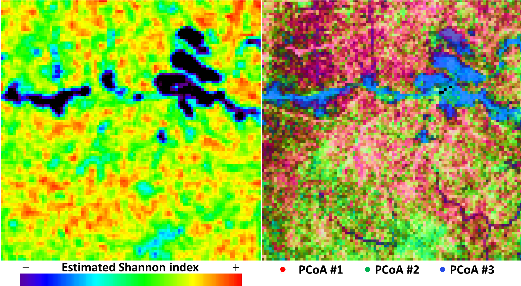
alpha and beta diversity maps

Jean-Baptiste Féret, Florian de Boissieu

2023-12-05

\(\alpha\) and \(\beta\) diversity maps are based on the SpectralSpecies raster.

The code to compute \(\alpha\) and \(\beta\) diversity maps from this file is as follows:

print("MAP ALPHA DIVERSITY")
# Index.Alpha   = c('Shannon','Simpson')
Index_Alpha <- c('Shannon')
map_alpha_div(Input_Image_File = Input_Image_File, 
              Output_Dir = Output_Dir, 
              TypePCA = TypePCA,
              window_size = window_size, 
              nbCPU = nbCPU, 
              MaxRAM = MaxRAM,
              Index_Alpha = Index_Alpha, 
              nbclusters = nbclusters)

print("MAP BETA DIVERSITY")
map_beta_div(Input_Image_File = Input_Image_File, 
             Output_Dir = Output_Dir, 
             TypePCA = TypePCA,
             window_size = window_size, 
             nbCPU = nbCPU, 
             MaxRAM = MaxRAM,
             nbclusters = nbclusters)

\(\alpha\) and \(\beta\) diversity maps are then stored in raster files located here:

RESULTS/S2A_T33NUD_20180104_Subset/SPCA/ALPHA

and here:

RESULTS/S2A_T33NUD_20180104_Subset/SPCA/BETA

Different types of rasters can be produced (full resolution or resolution defined with window_size). Users are invited to refer to the documentation for more options.

Here, processing our example leads to the following \(\alpha\) and \(\beta\) diversity maps:

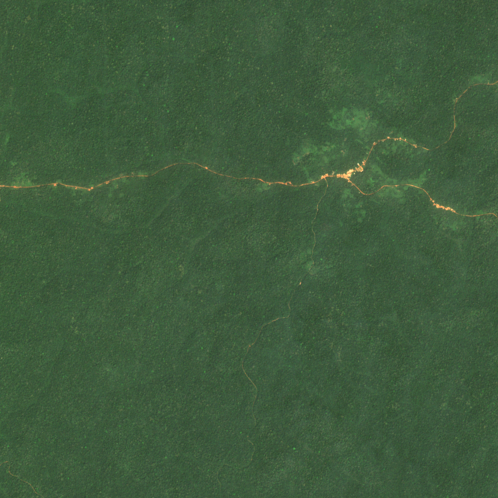
RGB representation of Sentinel-2 image.

Alternative diversity indices corresponding to functional diversity indices can also be computed. These do not require computation of the spectral species. They only require the PCA file or any stacked file.

The computation of teh functional diversity metrics is introduced in the next step.